1 Introduction

K - Nearest Neighbor is a supervised machine learning algorithm that classifies a new data point into the target class depending on the features of the neighboring data points. The objective of this paper is to demonstrate how the algorithm works using the R programming language. We will use the famous Iris dataset to run the algorithm.

1.1 Data Preparation

We need to do a few tasks first before running the KNN algorithm

Load necessary libraries
Read the data
Perform necessary wrangling tasks
Normalize the data

# load important packages
pacman::p_load(tidyverse, class, janitor, viridis, caret)


# read data
data("iris")

# view first 6 rows
head(iris)

ABCDEFGHIJ0123456789

	Sepal.Length <dbl>	Sepal.Width <dbl>	Petal.Length <dbl>	Petal.Width <dbl>	Species <fct>
1	5.1	3.5	1.4	0.2	setosa
2	4.9	3.0	1.4	0.2	setosa
3	4.7	3.2	1.3	0.2	setosa
4	4.6	3.1	1.5	0.2	setosa
5	5.0	3.6	1.4	0.2	setosa
6	5.4	3.9	1.7	0.4	setosa

# change column names into more readable names
iris <- iris %>% 
  clean_names()

# check names 
head(iris)

ABCDEFGHIJ0123456789

	sepal_length <dbl>	sepal_width <dbl>	petal_length <dbl>	petal_width <dbl>	species <fct>
1	5.1	3.5	1.4	0.2	setosa
2	4.9	3.0	1.4	0.2	setosa
3	4.7	3.2	1.3	0.2	setosa
4	4.6	3.1	1.5	0.2	setosa
5	5.0	3.6	1.4	0.2	setosa
6	5.4	3.9	1.7	0.4	setosa

Note that the variable species is our target variable.

# define a min-max normalize() function
# This function rescales a vector x such that its minimum value is zero and its maximum
# value is one; It does this by subtracting the minimum value from each value of x and
# dividing by the range of values of x.

normalize <- function(x){
  return((x - min(x)) / (max(x) - min(x)))
}

# apply normalization to the first 4 columns 
iris[, 1:4] <- normalize(iris[, 1:4])

head(iris)

ABCDEFGHIJ0123456789

	sepal_length <dbl>	sepal_width <dbl>	petal_length <dbl>	petal_width <dbl>	species <fct>
1	0.6410256	0.4358974	0.1666667	0.01282051	setosa
2	0.6153846	0.3717949	0.1666667	0.01282051	setosa
3	0.5897436	0.3974359	0.1538462	0.01282051	setosa
4	0.5769231	0.3846154	0.1794872	0.01282051	setosa
5	0.6282051	0.4487179	0.1666667	0.01282051	setosa
6	0.6794872	0.4871795	0.2051282	0.03846154	setosa

1.2 Data Splicing

We need to split the data into training and testing sets. We will use the training set to train the KNN algorithm and testing set to test the performance of the model. Lets use 80% of the data for training and the rest for testing.

# create a row id for each row
iris <- iris %>% 
  rowid_to_column()

# set seed for reproducible sampling 
set.seed(13745)

# split the data into training and testing sets
# apply the 80/20 splitting rule
training_set <- iris %>% 
  slice_sample(prop = 0.8)

# testing set
testing_set <- iris %>% 
  anti_join(training_set, by = "rowid")

1.3 Label creation and k value

k in general should be an odd number since the algorithm might confuse even number of classes.

# Assign row labels
species_type <- training_set$species

# Assign k to the rounded square root of the no. of observations in the training set
k_value <- round(sqrt(nrow(training_set)))

# print k_value
k_value

[1] 11

2 Model fitting

The knn() function from the class package is used to run the KNN algorithm.

predictions <- knn(
  # set train to training_set without rowid and species categories
  train = training_set %>% select(-c(rowid, species)),
  # set test to testing_set without rowid and species categories
  test = testing_set %>% select(-c(rowid, species)),
  # set class to training_set labels
  cl = species_type,
  # use the earlier define k_value as k
  k = k_value
)

head(predictions)

[1] setosa setosa setosa setosa setosa setosa
Levels: setosa versicolor virginica

3 Plotting Values

Lets add the predictions to our testing_set as follows

# define plotting data
plotting_data <- testing_set %>% 
  # rename species variable to actual_species
  rename(actual_species = species) %>% 
  # add knn predictions as a variable as predicted_species
  mutate(predicted_species = predictions)

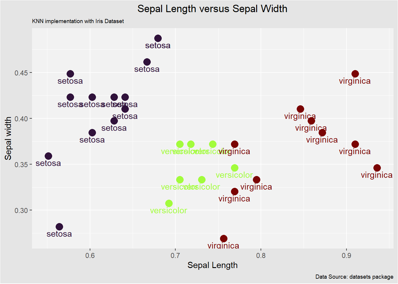
we can utilize a scatter plot to visualize the relationship between sepal length and sepal width as follows

# make a scatter plot of sepal length vs sepal width
plotting_data %>% 
  ggplot(aes(
    sepal_length, 
    sepal_width,
    color = predicted_species,
    fill = predicted_species)
    )+
  geom_point(size = 4, show.legend = F)+
  geom_text(
    aes(label = actual_species, hjust = .5, vjust = 1.5)
    ) +
  labs(
    x = "Sepal Length",
    y = "Sepal width",
    title = "Sepal Length versus Sepal Width",
    subtitle = "KNN implementation with Iris Dataset",
    caption = "Data Source: datasets package"
  )+
  scale_color_viridis(discrete = TRUE, option = "turbo")+
  scale_fill_viridis(discrete = TRUE)+
  theme(
    legend.position = "none",
    plot.background = element_rect(fill = "gray90"),
    panel.background = element_rect(fill = "gray95"),
    plot.title = element_text(hjust = 0.5),
    plot.caption = element_text(size = 7),
    plot.subtitle = element_text(size = 7)
  )

Warning

Note that some data points have been incorrectly classified as type virginica instead of versicolor.

We can also visualize the relationship between the petal length and petal width as follows

# make a scatter plot of sepal length vs sepal width
plotting_data %>% 
  ggplot(aes(
    petal_length, 
    petal_width,
    color = predicted_species,
    fill = predicted_species)
    )+
  geom_point(size = 4, show.legend = F)+
  geom_text(
    aes(label = actual_species, hjust = .5, vjust = 1.5)
    ) +
  labs(
    x = "Petal Length",
    y = "Petal width",
    title = "Petal Length versus Petal Width",
    subtitle = "KNN implementation with Iris Dataset",
    caption = "Data Source: datasets package"
  )+
  scale_color_viridis(discrete = TRUE, option = "turbo")+
  scale_fill_viridis(discrete = TRUE)+
  theme(
    legend.position = "none",
    plot.background = element_rect(fill = "gray90"),
    panel.background = element_rect(fill = "gray95"),
    plot.title = element_text(hjust = 0.5),
    plot.caption = element_text(size = 7),
    plot.subtitle = element_text(size = 7)
  )

In this case, the algorithm does well in classifying each data point to the target class.

4 Model Accuracy

After building the model, it is time to evaluate its accuracy. We will use the confusionMatrix() function from the caret package to generate the confusion matrix and calculate statistics.

# generate confusion matrix and model statistics 
confusionMatrix(table(predictions, testing_set$species))

Confusion Matrix and Statistics

            
predictions  setosa versicolor virginica
  setosa         13          0         0
  versicolor      0          7         0
  virginica       0          0        10

Overall Statistics
                                     
               Accuracy : 1          
                 95% CI : (0.8843, 1)
    No Information Rate : 0.4333     
    P-Value [Acc > NIR] : 1.273e-11  
                                     
                  Kappa : 1          
                                     
 Mcnemar's Test P-Value : NA         

Statistics by Class:

                     Class: setosa Class: versicolor Class: virginica
Sensitivity                 1.0000            1.0000           1.0000
Specificity                 1.0000            1.0000           1.0000
Pos Pred Value              1.0000            1.0000           1.0000
Neg Pred Value              1.0000            1.0000           1.0000
Prevalence                  0.4333            0.2333           0.3333
Detection Rate              0.4333            0.2333           0.3333
Detection Prevalence        0.4333            0.2333           0.3333
Balanced Accuracy           1.0000            1.0000           1.0000

# put the results into tidy format
confusionMatrix(table(predictions, testing_set$species)) %>% 
  broom::tidy()

ABCDEFGHIJ0123456789

term <chr>	class <chr>	estimate <dbl>	conf.low <dbl>	conf.high <dbl>
accuracy	NA	1.0000000	0.8842967	1
kappa	NA	1.0000000	NA	NA
mcnemar	NA	NA	NA	NA
sensitivity	setosa	1.0000000	NA	NA
specificity	setosa	1.0000000	NA	NA
pos_pred_value	setosa	1.0000000	NA	NA
neg_pred_value	setosa	1.0000000	NA	NA
precision	setosa	1.0000000	NA	NA
recall	setosa	1.0000000	NA	NA
f1	setosa	1.0000000	NA	NA

So, from the output, we can see that our model predicts the outcome with an accuracy of 86.67% which is good since we worked with a small data set. A point to remember is that the more data (optimal data) we feed the machine, the more efficient the model will be.